B Informations supplémentaires
Article 1
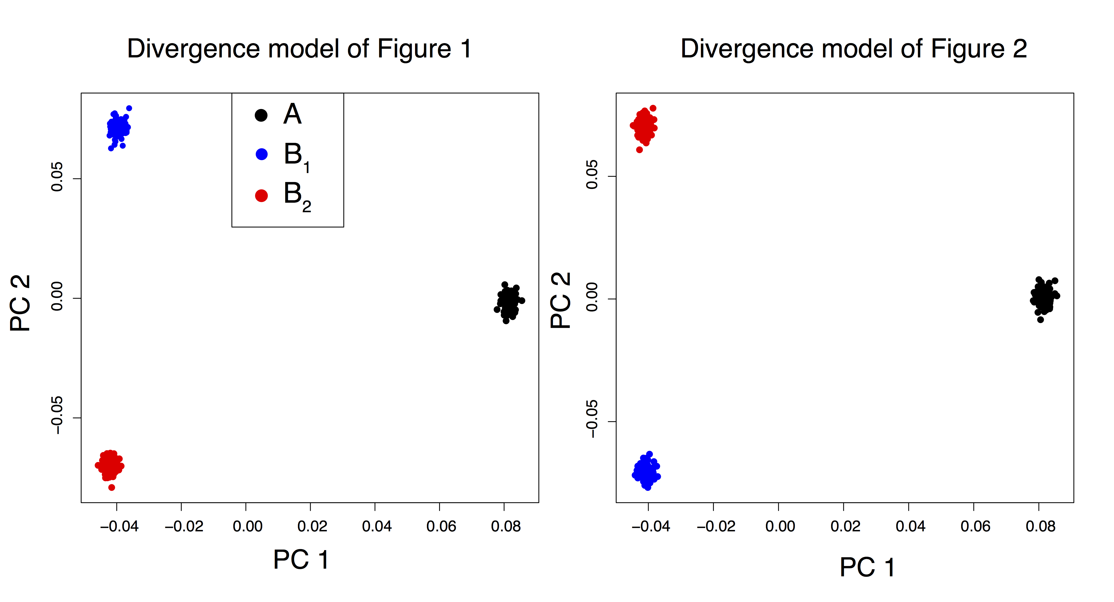
Figure B.1: Principal component analysis for SNP data simulated under the divergence model depicted in Figures 1 and 2 of the main text.
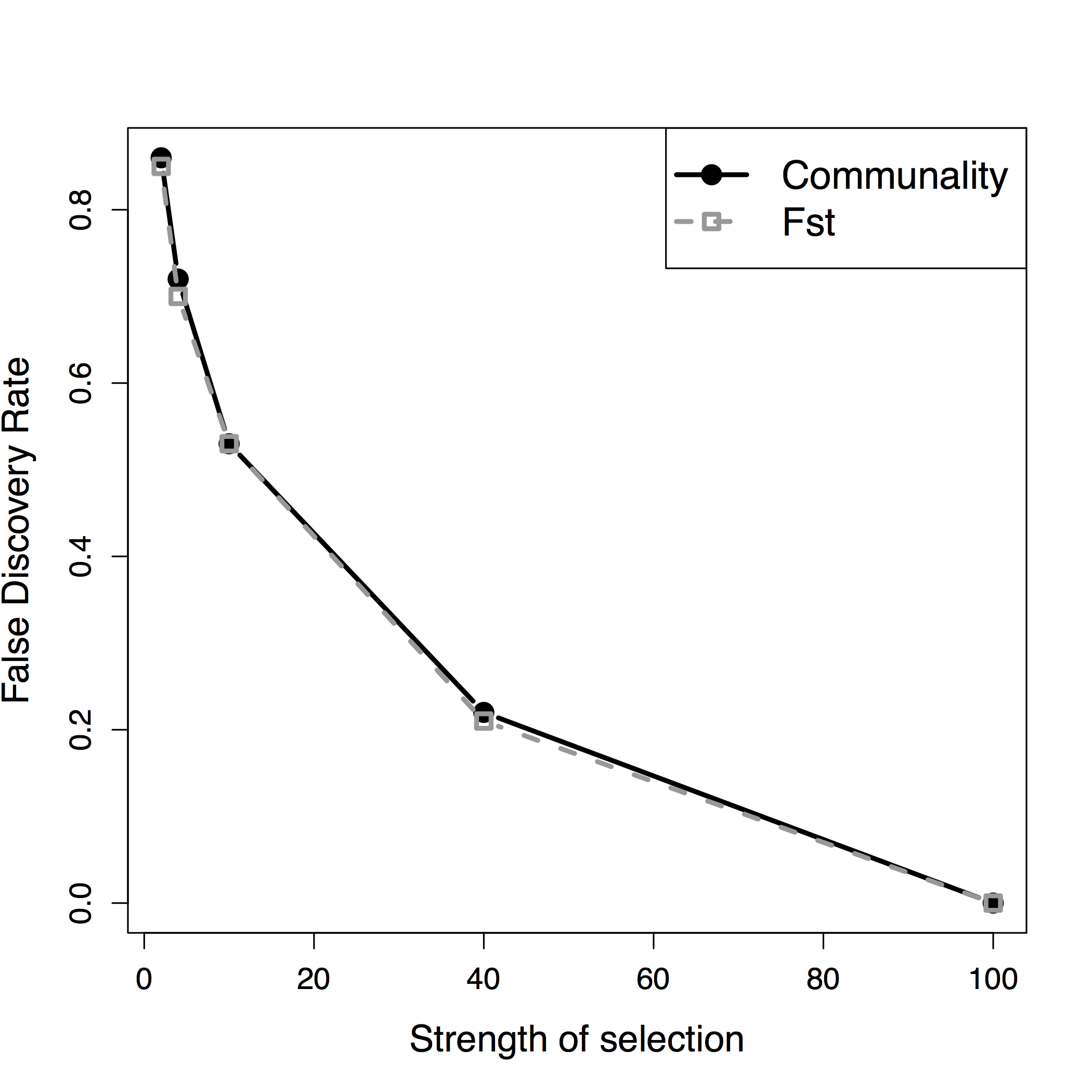
Figure B.2: False discovery rate of the 1% top-ranked SNPs obtained with \(h^2\) and with \(F_{ST}\) under an island model.
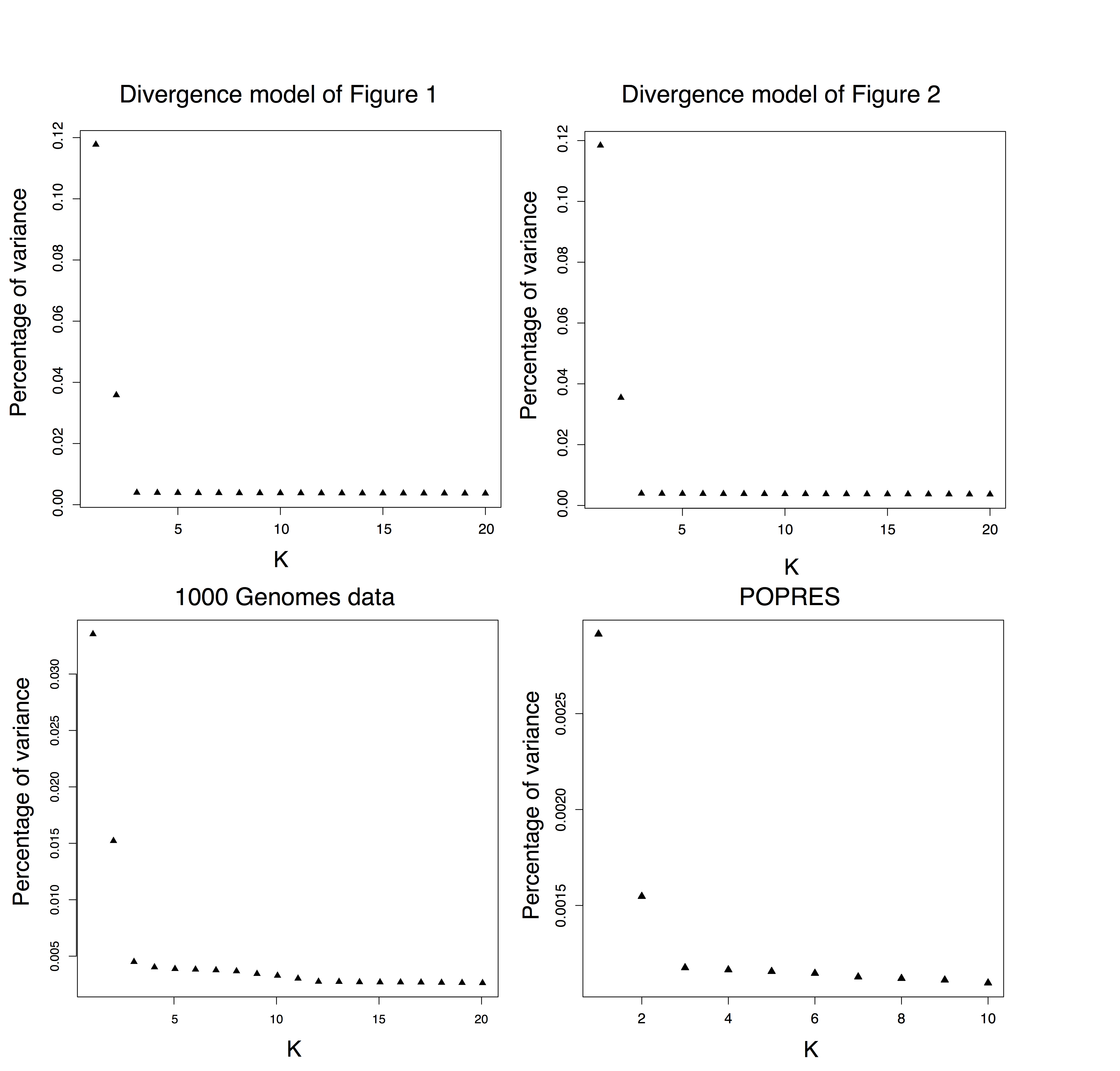
Figure B.3: Decay of eigenvalues of the covariance matrix for divergence models, the 1000 Genome data, and POPRES.
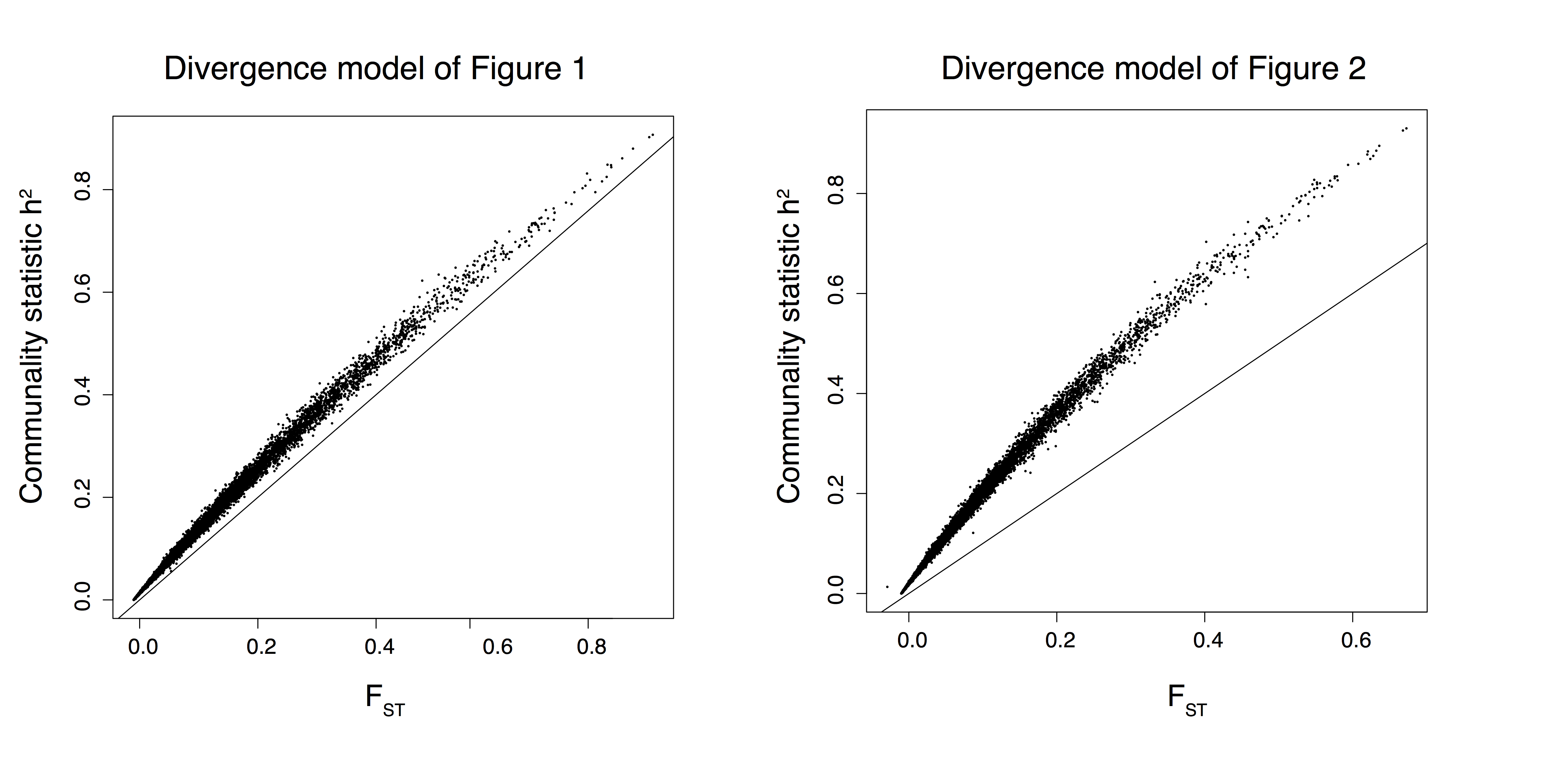
Figure B.4: Communality statistic as a function of \(F_{ST}\) for SNPs simulated with a divergence model.
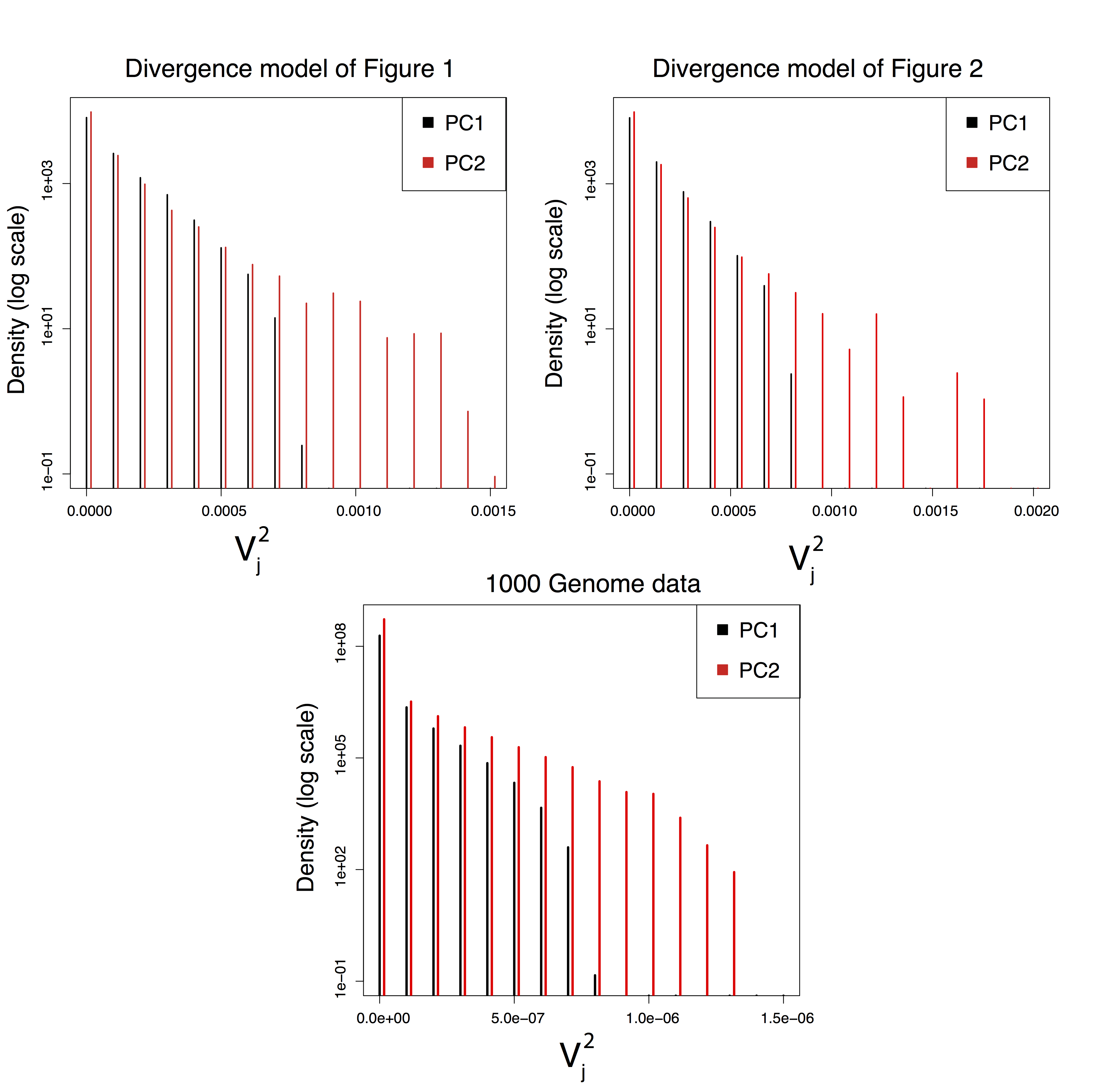
Figure B.5: Histograms of the squared normalized loadings \(V_{jk}^2\), \(k = 1, 2\), obtained for SNPs simulated with divergence models and for SNPs of the 1000 Genomes data.
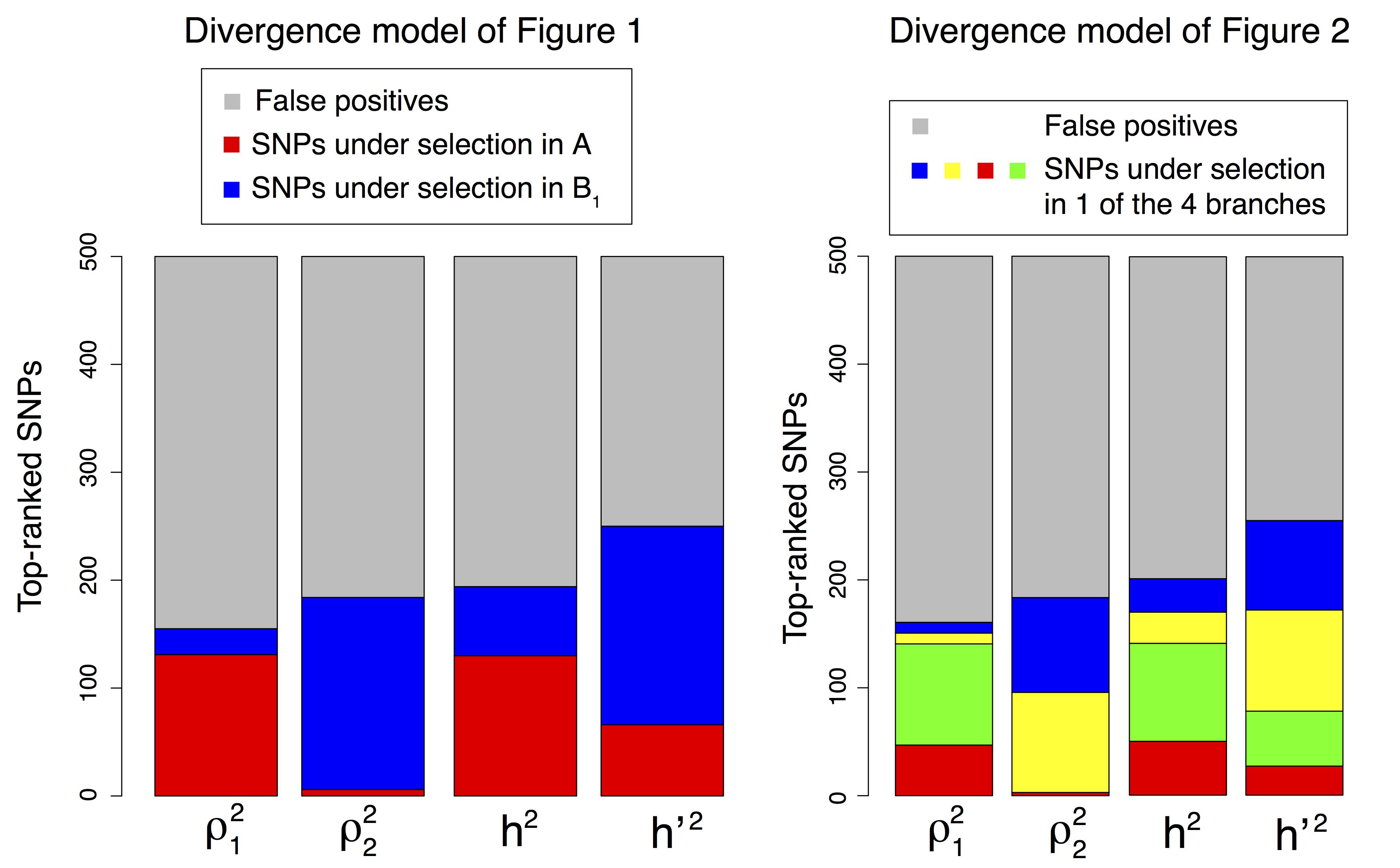
Figure B.6: Repartition of the 5% top-ranked SNPs of each PCA-based statistic under the two divergence models.
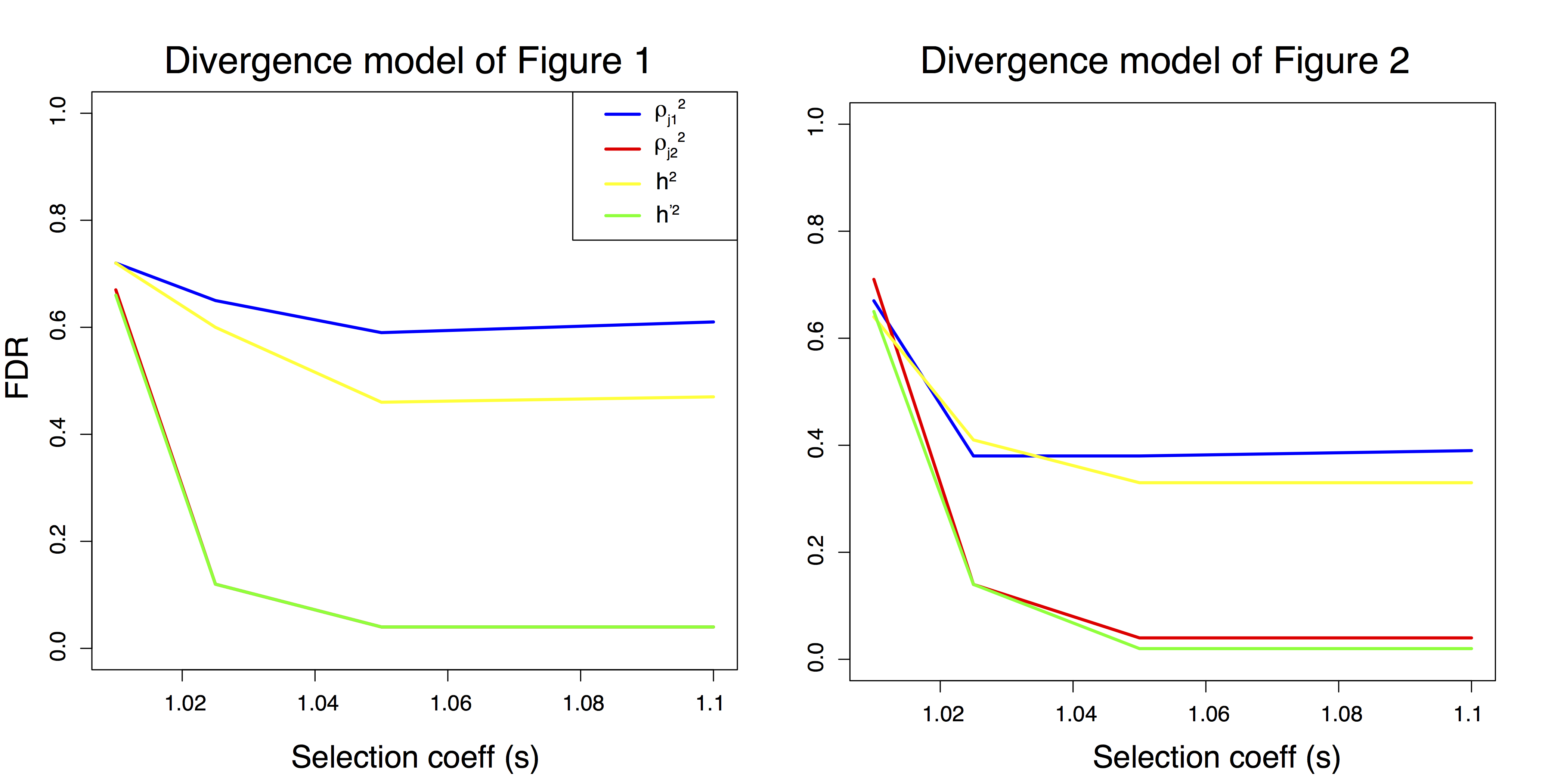
Figure B.7: False discovery rate as a function of the selection coefficient under the two divergence models.
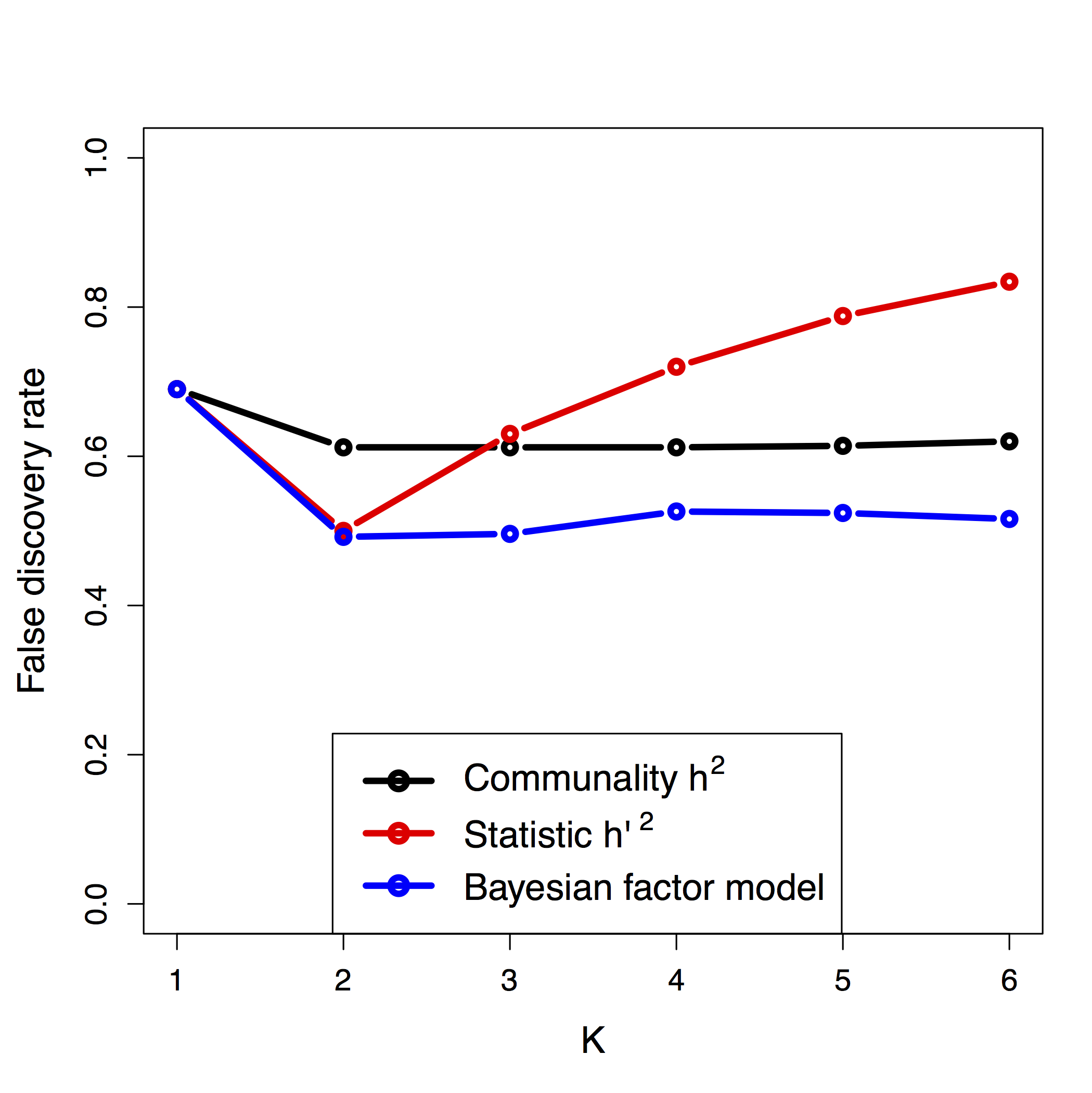
Figure B.8: False discovery rate as a function of the number \(K\) of principal components under the two divergence models.
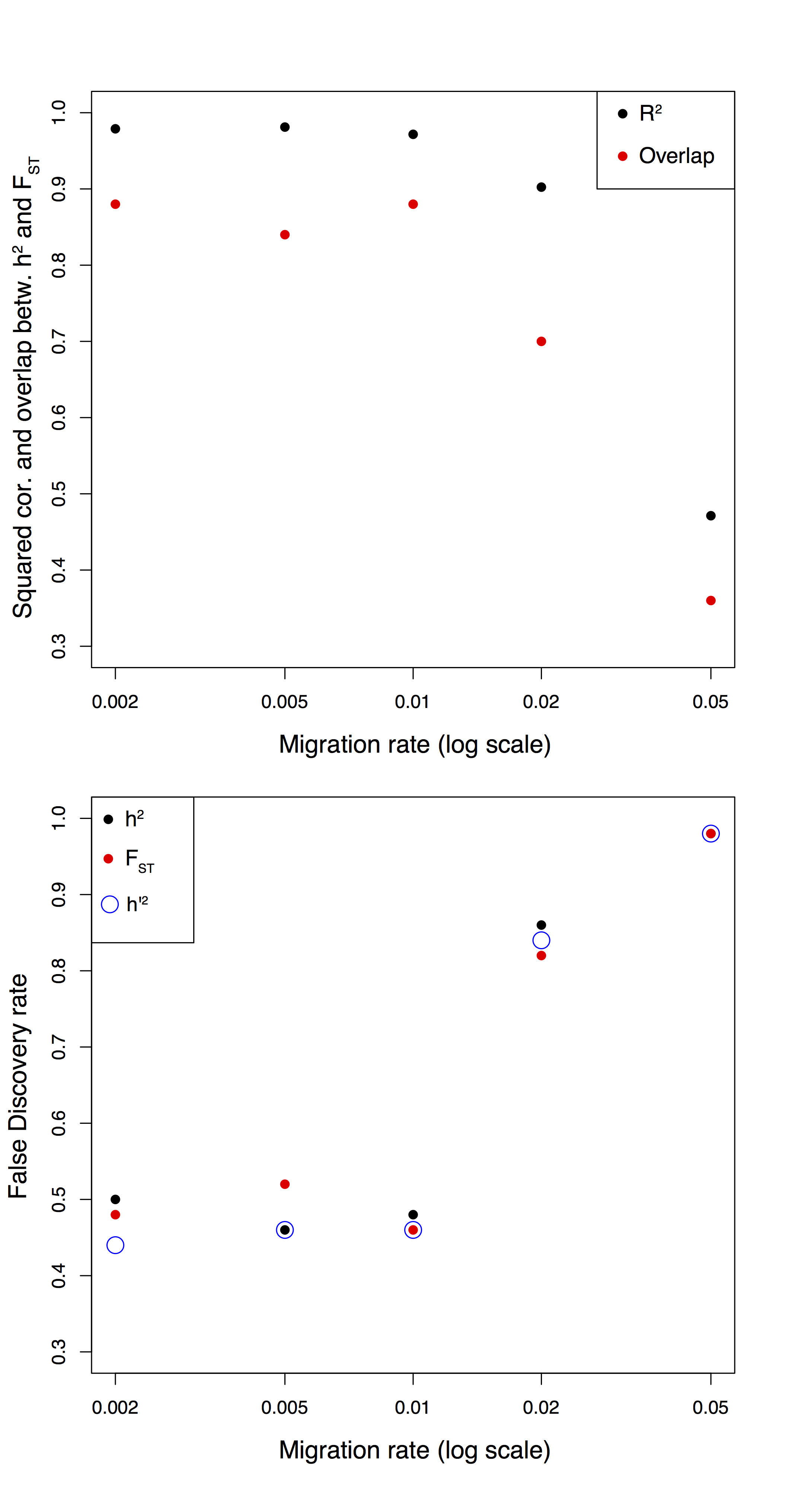
Figure B.9: Comparison between \(h^2\) and \(F_{ST}\) in a isolation-with-migration model.
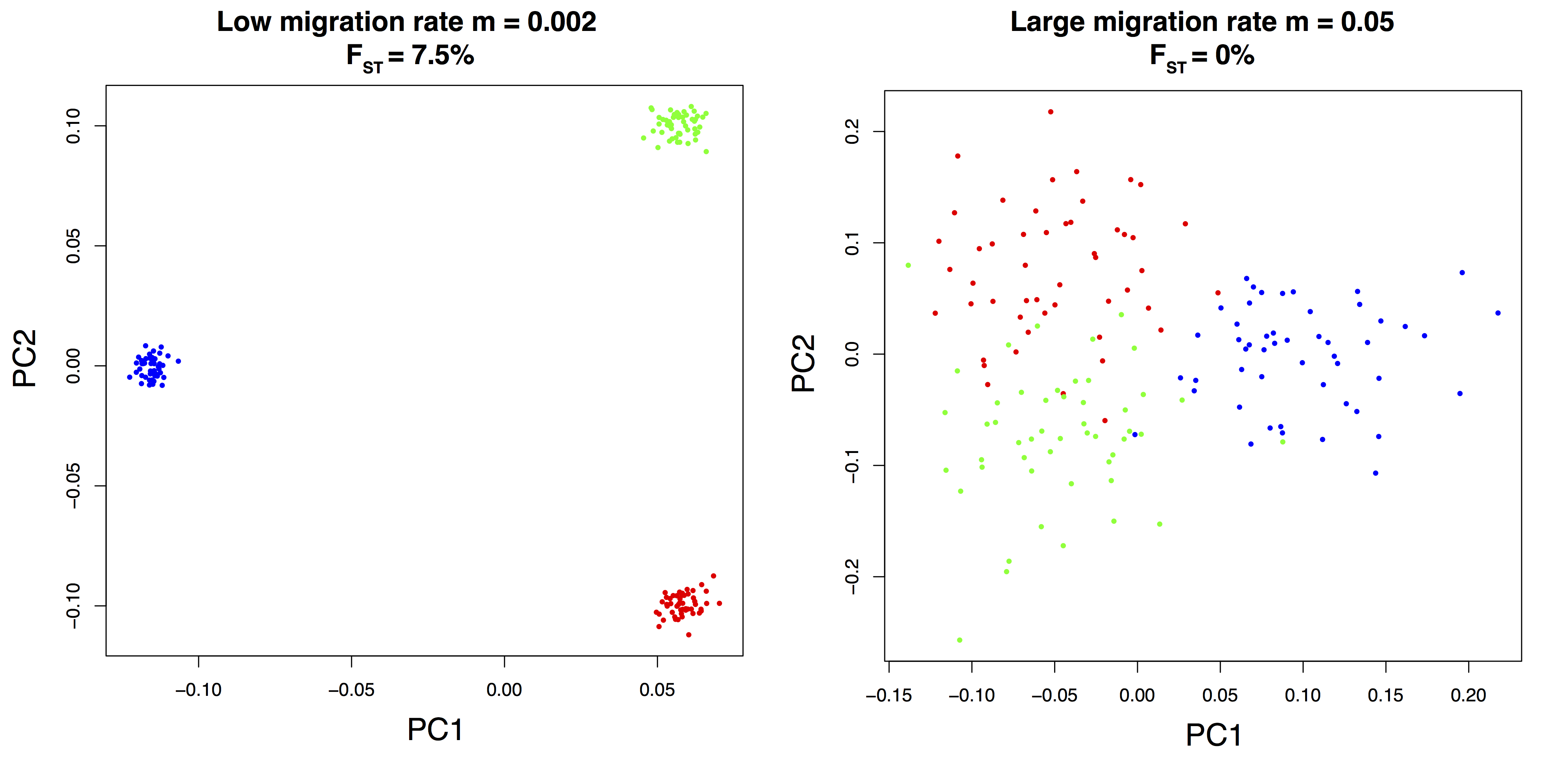
Figure B.10: Principal component analysis of SNPs simulated with an isolation-with-migration model.
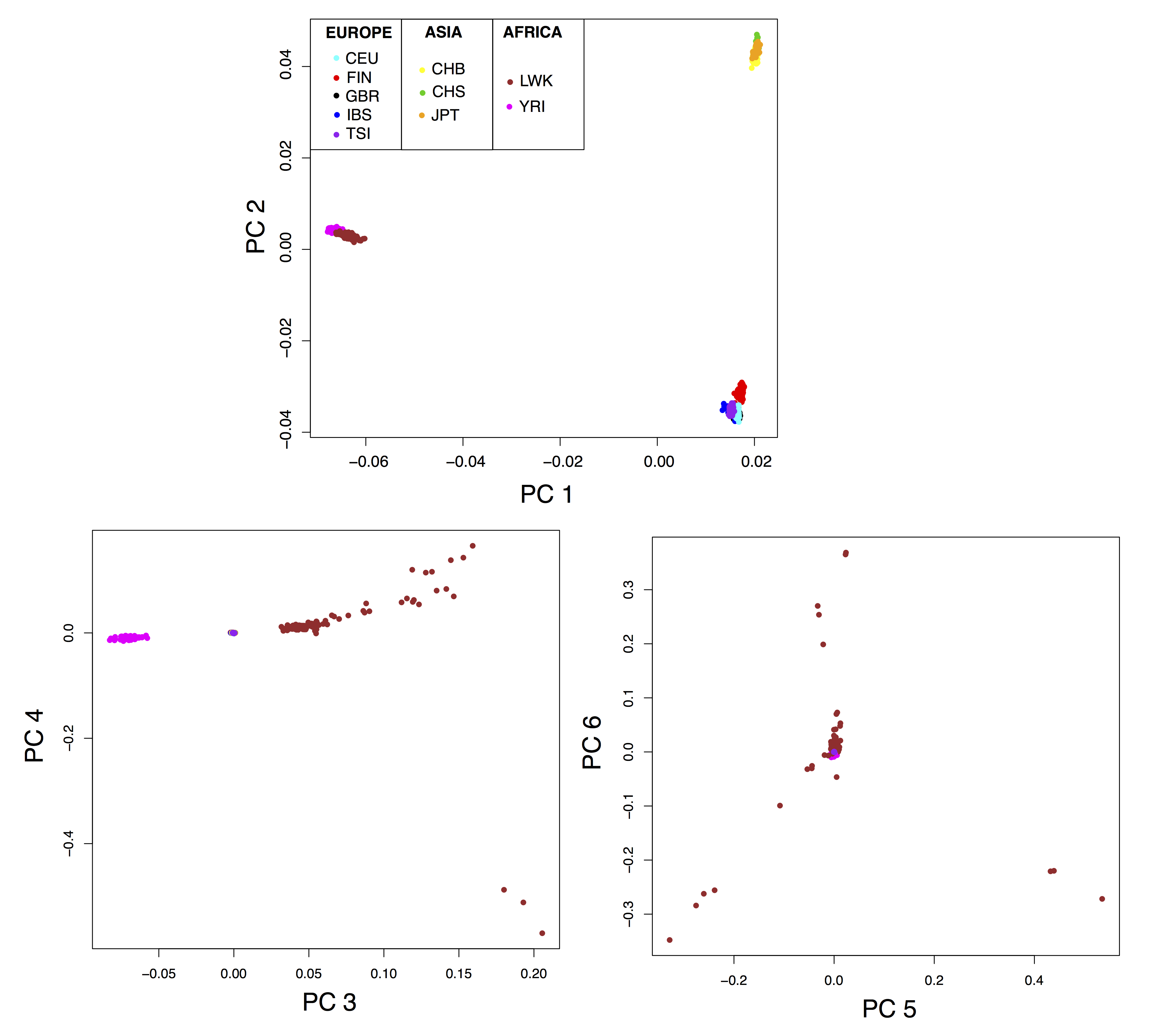
Figure B.11: Principal component analysis of the 1000 Genome data.
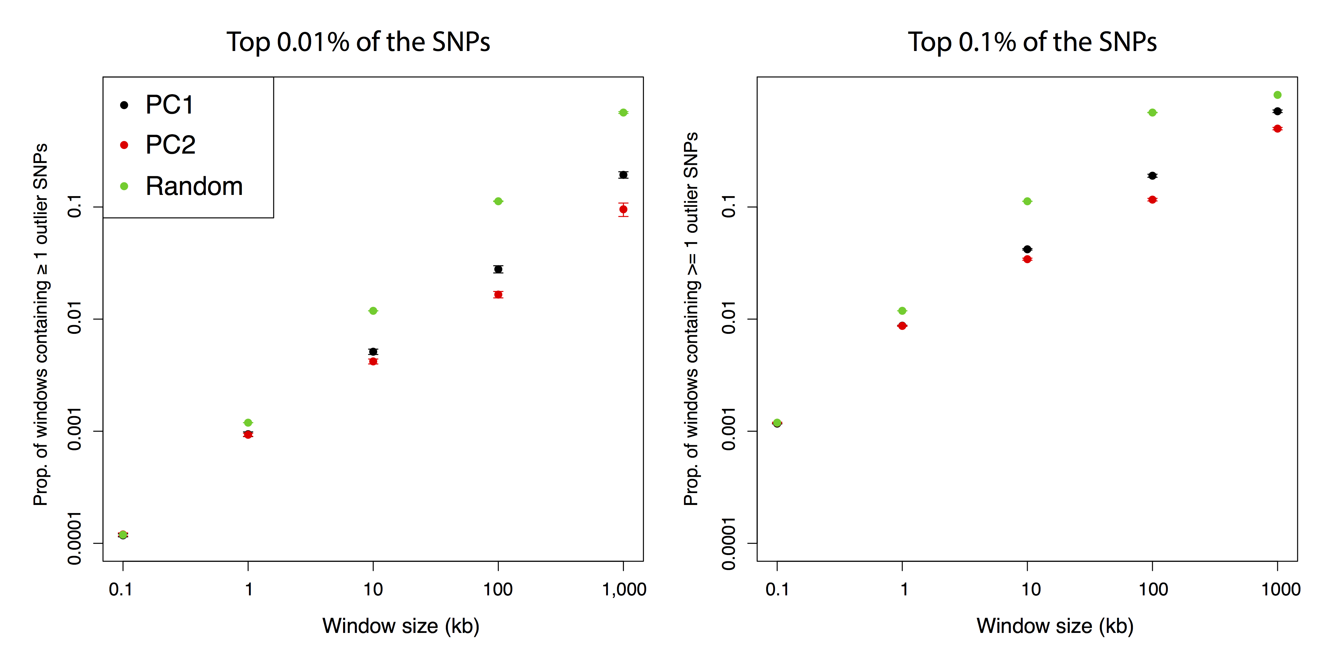
Figure B.12: Number of contiguous windows containing one or more outlier SNPs.
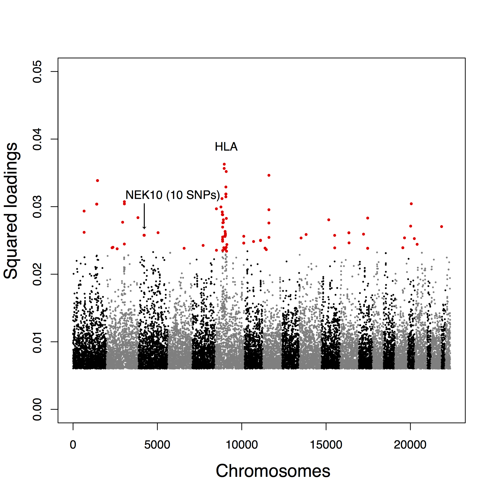
Figure B.13: Manhattan plot for the POPRES data of the squared loadings \(\rho_{j2}^2\) with the second principal component.
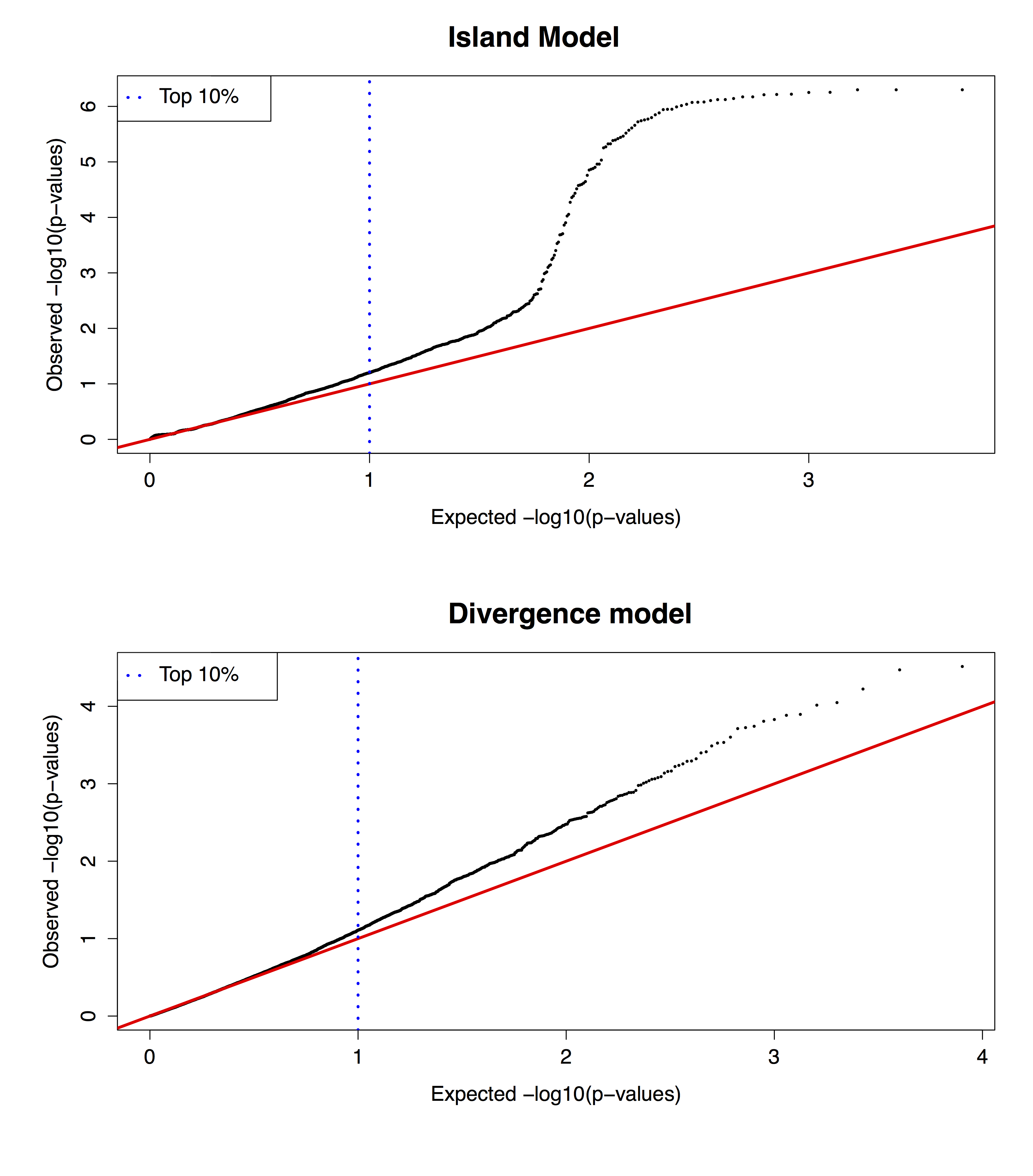
Figure B.14: Q-Q plots of the \(P\)-values, which are based on the communality \(h^2\) statistic, under an island and a divergence model.
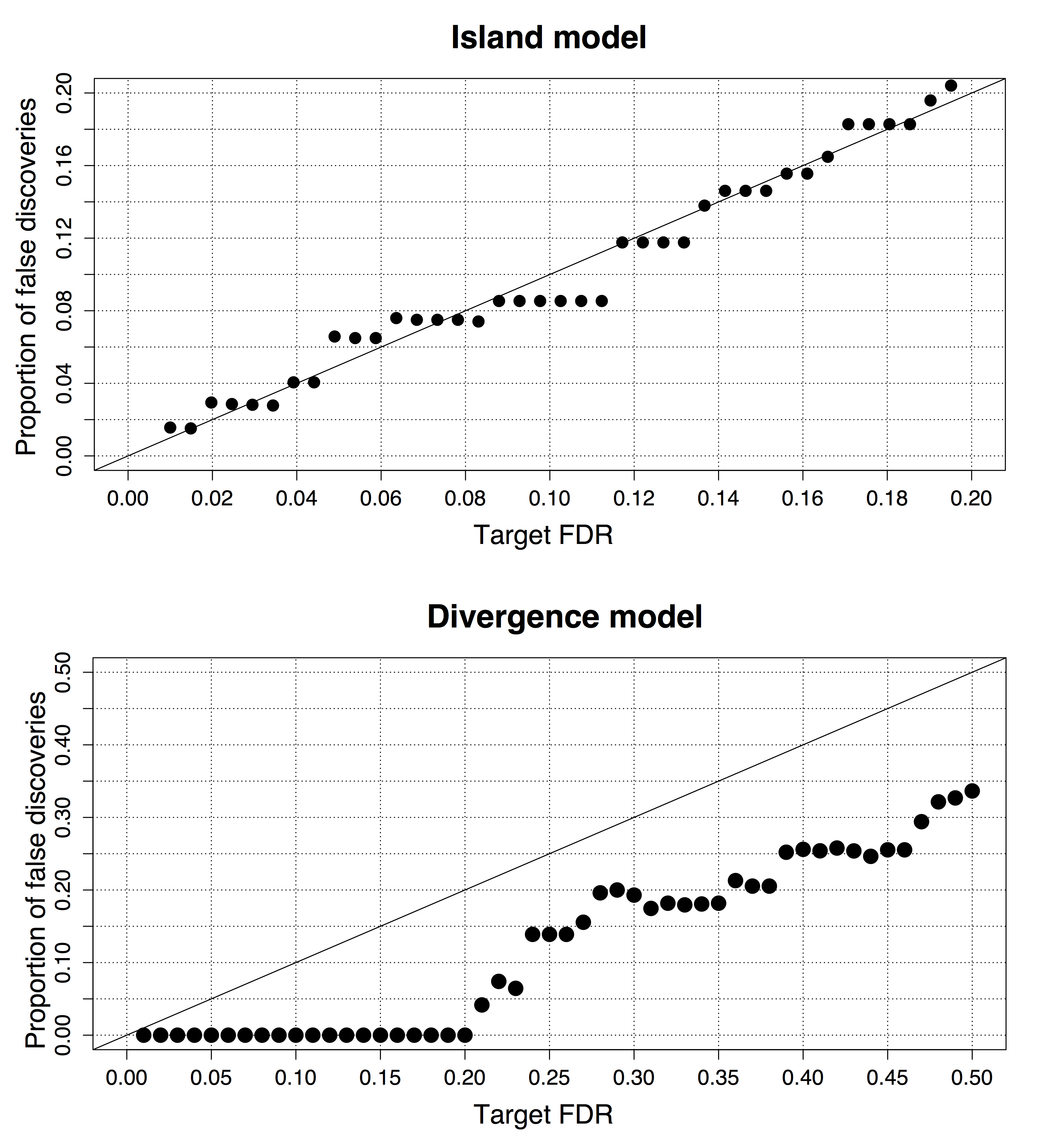
Figure B.15: Control of the false discovery rate for SNPs simulated under an island and a divergence model.
Article 2
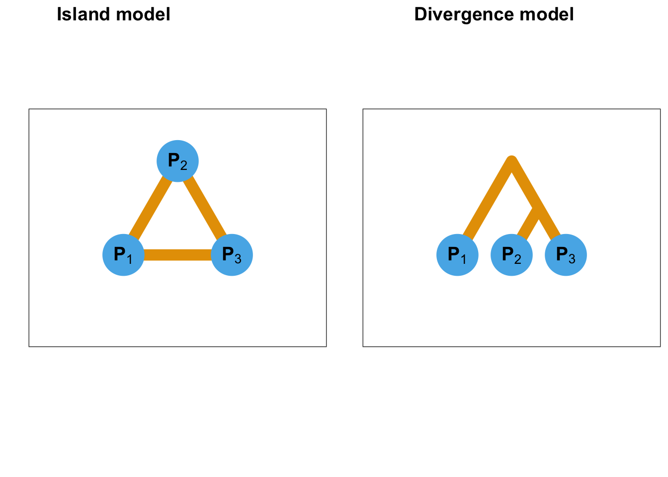
Figure B.16: Schematic description of the island and divergence model. For the island model, adaptation occurs simultaneously in each population. For the divergence model, adaptation takes place in the branch leading to the second population.
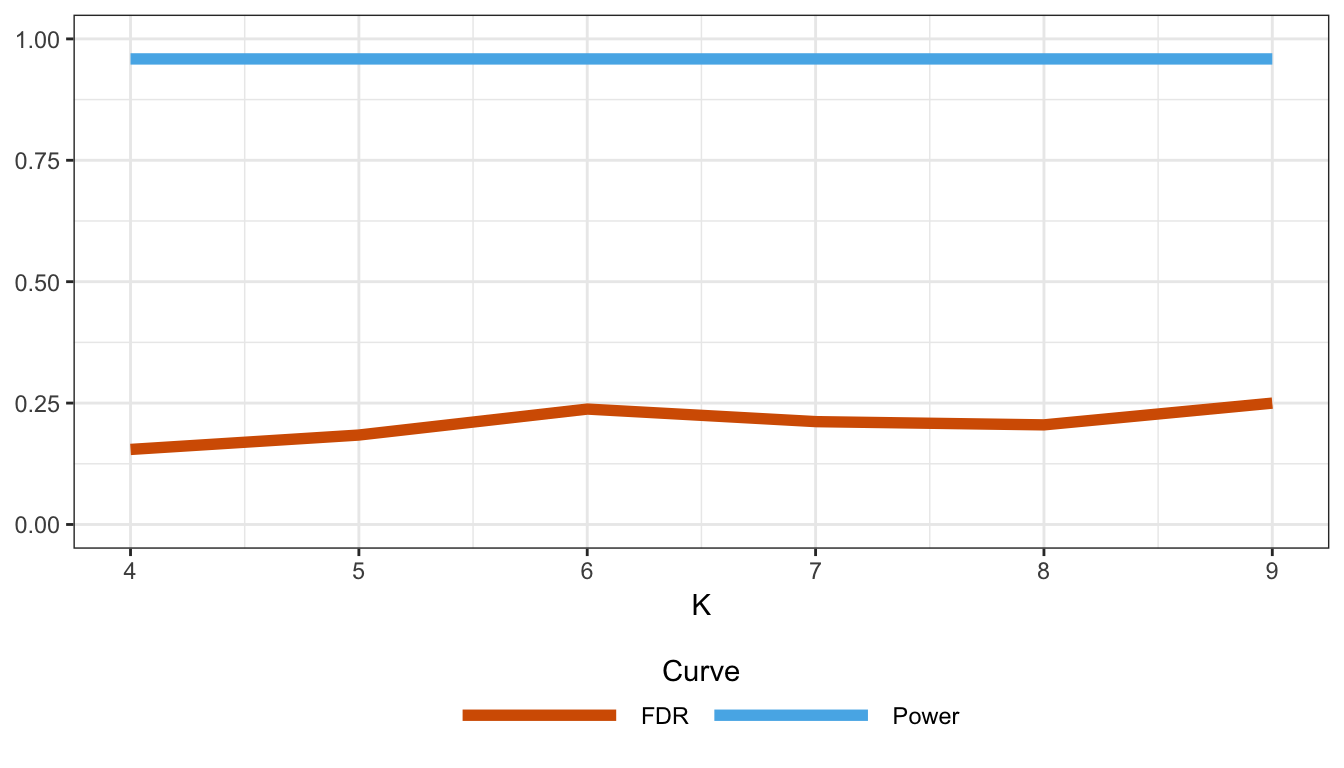
Figure B.17: Proportion of false discoveries and statistical power as a function of the number of principal components in a model of range expansion.
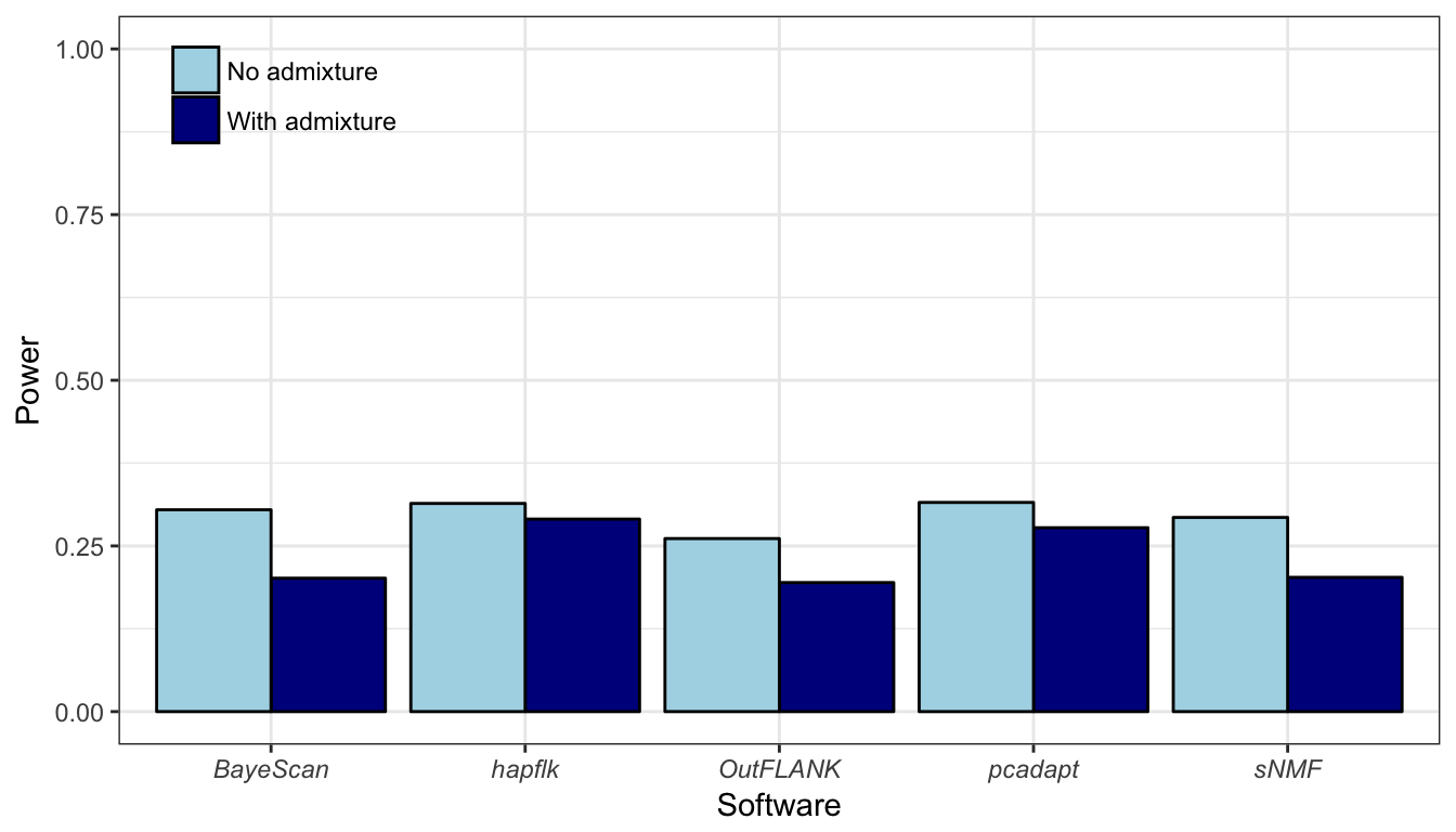
Figure B.18: Statistical power averaged over the expected proportion of false discoveries (ranging between 0% and 50%) for the island model.
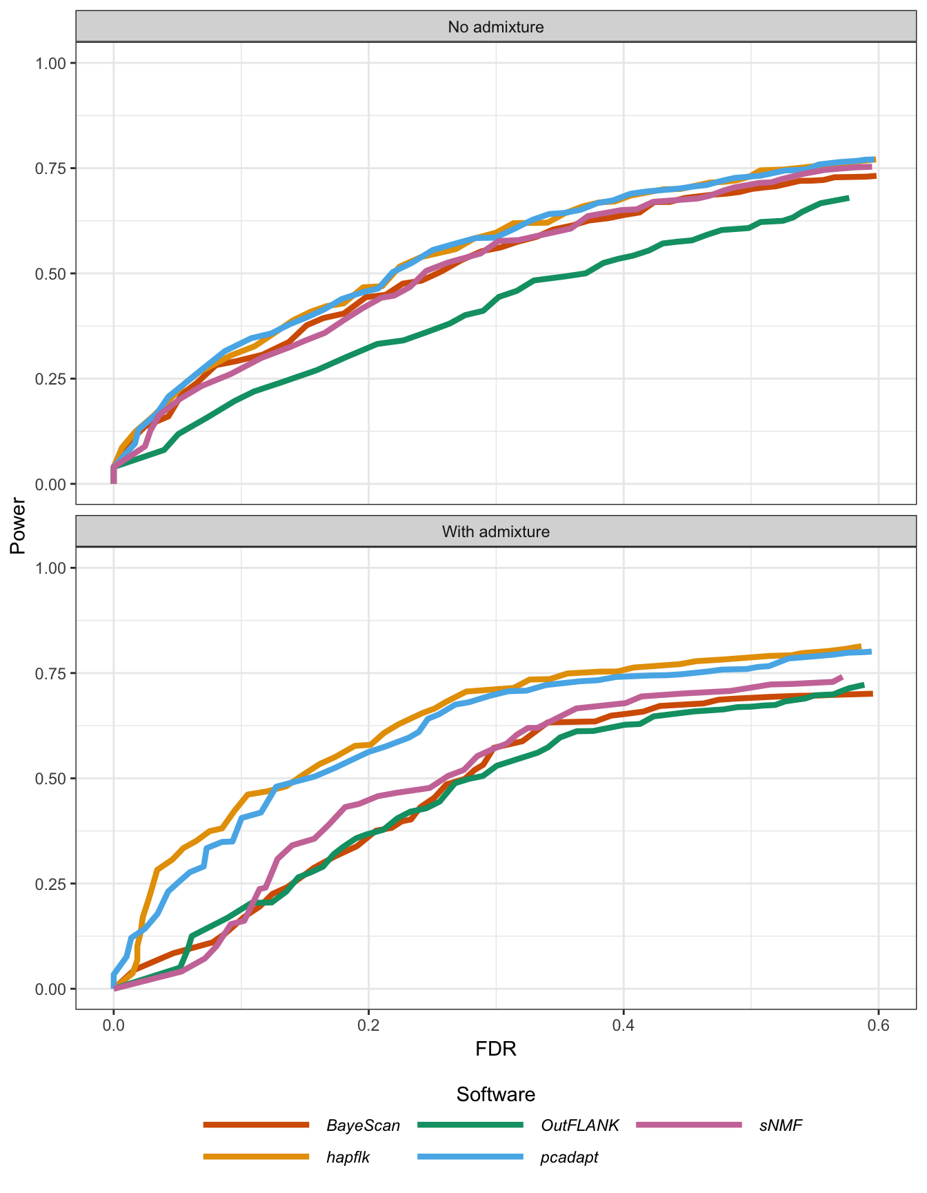
Figure B.19: Statistical power as a function of the proportion of false discoveries for the island model.
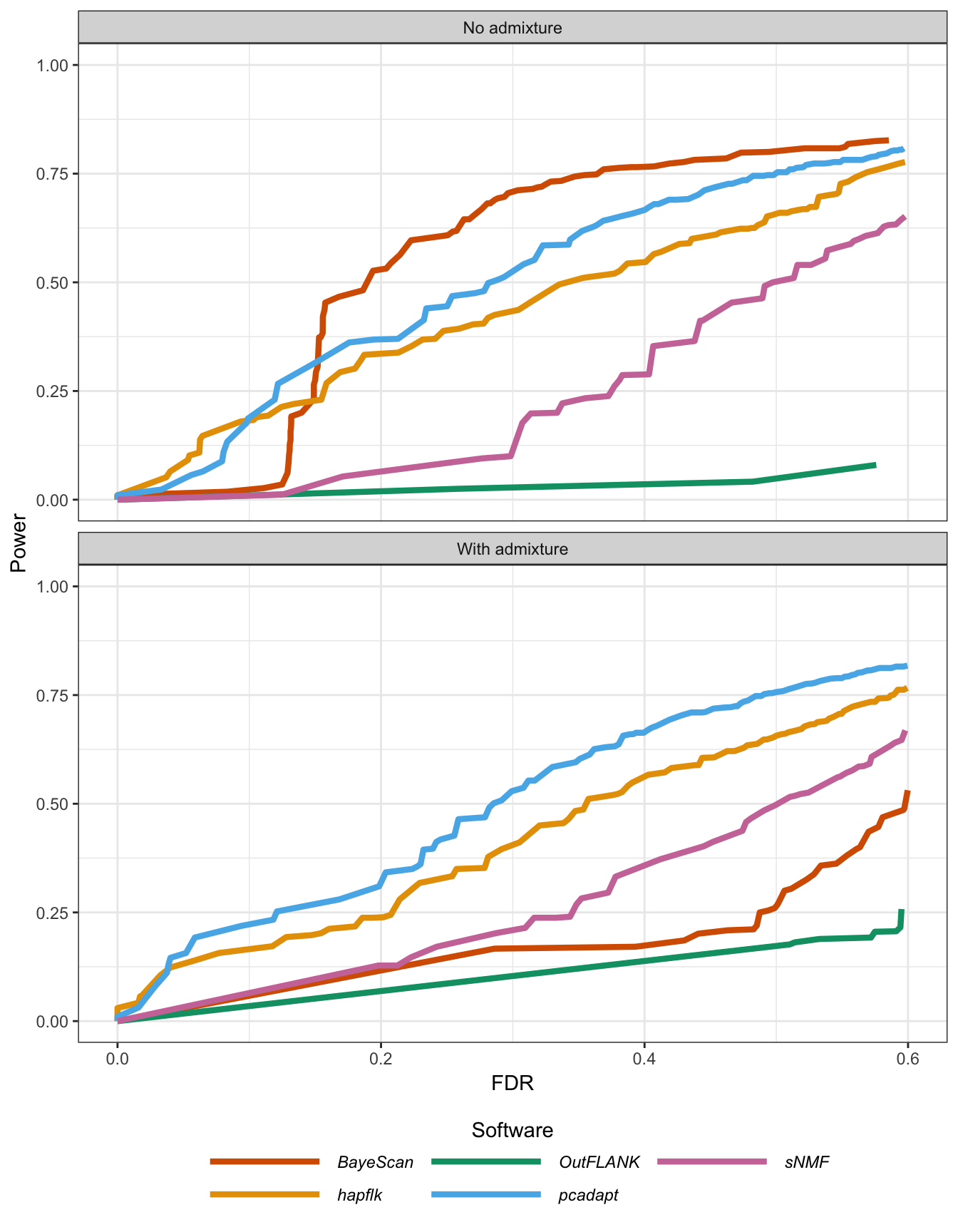
Figure B.20: Statistical power as a function of the proportion of false discoveries for the divergence model.
Figure B.21: Statistical power as a function of the proportion of false discoveries for the model of range expansion.
Figure B.22: Running times of the different computer programs. The different programs were run on genotype matrices containing 300 individuals and from 500 to 50,000 SNPs. The characteristics of the computer we used to perform comparisons are the following: OSX El Capitan 10.11.3, 2,5 GHz Intel Core i5, 8 Go 1600 MHz DDR3.
Article 3
Figure B.23: Standardized average ancestry coefficient computed with pcadapt and different LAI methods (EILA, Loter and RFMix) for a population of simulated admixed individuals. Simulations use phased genotype data from \(25\) Populus balsamifera individuals and \(25\) Populus trichocarpa individuals and assume that admixture took place \(\lambda=100\) generations ago. A total of \(25\) admixed individuals were generated assuming \(30\%\) of Populus balsamifera ancestry except from the 5 outlier \(500\) SNP regions where Populus balsamifera ancestry is of \(50\%\).
Figure B.24: Relative loss of power of the different methods when compared to an ideal method called oracle, which would know ancestry chunks for each admixed individual. The relative power is averaged over the difference \(\Delta_q\) of ancestry between neutral and outlier regions. Simulations use phased genotype data from \(25\) Populus balsamifera individuals and \(25\) Populus trichocarpa individuals and assume that admixture took place \(\lambda\) generations ago. A total of \(25\) admixed individuals were generated assuming \(70\%\) of Populus balsamifera ancestry except from the 5 outlier \(500\) SNP regions where Populus balsamifera ancestry is of \(70\%-\Delta_q\) where \(\Delta_q\) is equal to \(0.05\), \(0.10\), \(0.15\), \(0.20\), \(0.30\), \(0.40\), or \(0.50\).
Figure B.25: Proportion of true outlier peaks among the five top peaks found with pcadapt and different LAI methods (EILA, Loter and RFMix) in a scenario where 2 Populus populations experienced admixture. Compared to Figure 3.10, we compute maximum of ancestry coefficients within each genomic region instead of mean of ancestry coefficients. Proportion of true outlier peaks are displayed as a function of the difference \(\Delta_q\) of ancestry between outlier and neutral regions. The three panels correspond to the three different possible values (\(\lambda=10\) or \(100\) or \(1000\)) of the number of generations since admixture.
Figure B.26: Proportion of true outlier peaks as a function of the number of top peaks found with pcadapt and different LAI methods (EILA, Loter and RFMix) in a scenario where 2 Populus populations experienced admixture. The different panels correspond to the different possible values for the number of generations since admixture occurred (\(\lambda=\{10,100,1000\}\)) and to the different values of the difference of ancestry \(\Delta_q\) between neutral and outlier regions.
Figure B.27: Power as a function of the proportion of introgression.
Figure B.28: Schematic description of simulations under an introgression scenario.
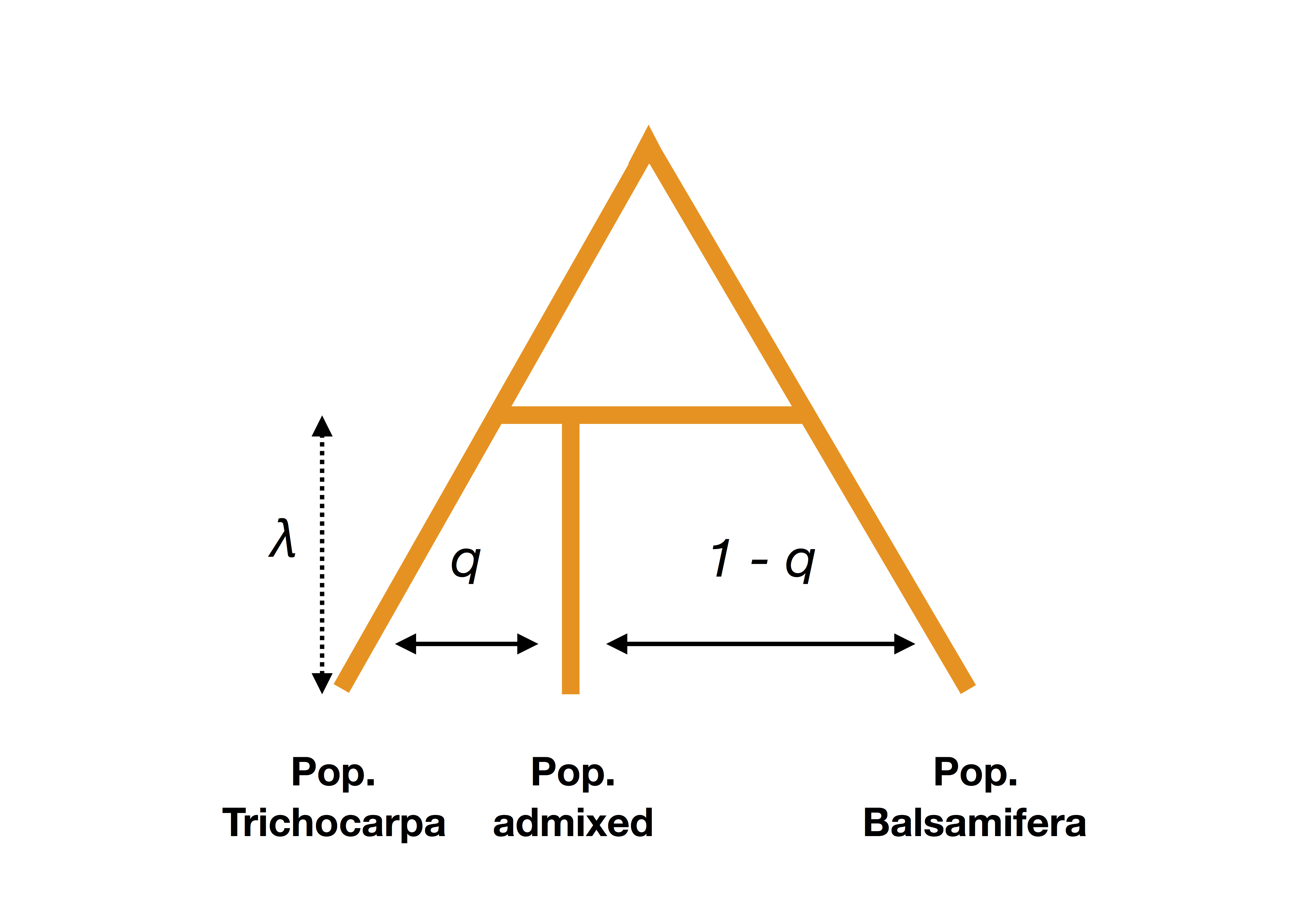
Figure B.29: Schematic description of simulations under an admixture scenario.